Reference Junction Compensation in Thermocouple
Multiple techniques exist to deal with the influence of the reference junction’s temperature. One technique is to physically fix the temperature of that junction at some constant value so it is always stable.
This way, any changes in measured voltage must be due to changes in temperature at the measurement junction, since the reference junction has been rendered incapable of changing temperature.
This may be accomplished by immersing the reference junction in a bath of ice and water, the ice/water mixture ensuring a stable temperature by means of water’s latent heat of fusion:
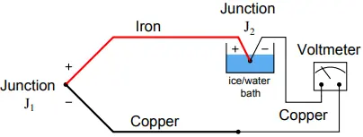
In fact, this is how thermocouple temperature/voltage tables are referenced: describing the amount of voltage produced for given temperatures at the measurement junction with the reference junction held at the freezing point of water (0 oC = 32oF).
With the reference junction maintained at the freezing point of water, and thermocouple tables referenced to that specific cold junction temperature, the voltmeter’s indication will simply and directly correspond to the temperature of measurement junction J1 at all times.
However, fixing the reference junction at the temperature of freezing water is impractical for any real thermocouple application outside of a laboratory.
Instead, we need to find some other way to compensate for changes in reference junction temperature, so that we may accurately interpret the temperature of the measurement junction despite random changes in reference junction temperature.
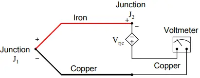
A practical way to compensate for the reference junction voltage is to include an additional voltage source within the thermocouple circuit equal in magnitude and opposite in polarity to the reference junction voltage.
If this additional voltage is made continually equal to the reference junction’s potential, it will precisely counter the reference junction voltage, resulting in the full (measurement junction) voltage appearing at the measuring instrument terminals.
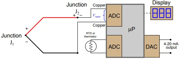
This is called a reference junction compensation or cold junction compensation circuit:
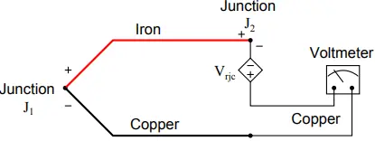
In order for such a compensation strategy to work, the compensating voltage must continuously track the voltage produced by the reference junction.
To do this, the compensating voltage source (Vrjc in the above schematic) uses some other temperature-sensing device such as a thermistor or RTD to sense the local temperature at the terminal block where junction J2 is formed and produce a counter-voltage that is precisely equal and opposite to J2’s voltage (Vrjc = VJ2) at all times.
Having canceled the effect of the reference junction, the voltmeter now only registers the voltage produced by the measurement junction J1: Vmeter = VJ1 − VJ2 + Vrjc
Vmeter = VJ1 + 0 (If Vrjc = VJ2)
Vmeter = VJ1
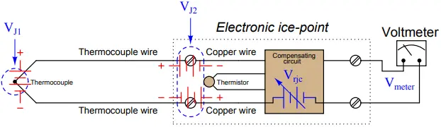
Some instrument manufacturers sell electronic ice point modules designed to provide reference junction compensation for un-compensated instruments such as standard voltmeters.
The “ice point” circuit performs the function shown by Vrjc in the previous diagram: it inserts a counter-acting voltage to cancel the voltage generated by the reference junction, so that the voltmeter only “sees” the measurement junction’s voltage.
This compensating voltage is maintained at the proper value according to the terminal temperature where the thermocouple wires connect to the ice point module, sensed by a thermistor or RTD:
Example values:
TJ1 = 570 oF (type J), TJ2 = 69 oF (type J)
VJ1 = 16.266 mV, VJ2 = 1.048 mV
Vrjc = 1.048 mV
Vmeter = VJ1 – VJ2 + Vrjc
Vmeter = 16.266 mV – 1.048 mV + 1.048 mV
Vmeter = 16.266 mV (equivalent to 570 oF)
In this example, we see the measurement junction (J1) at a temperature of 570 degrees Fahrenheit, generating a voltage of 16.266 millivolts.
If this thermocouple were directly connected to the meter, the meter would only register 15.218 millivolts, because the reference junction (J2, at 69 degrees Fahrenheit) opposes with its own voltage of 1.048 millivolts.
With the ice point compensation circuit installed, however, the 1.048 millivolts of the reference junction is canceled by the ice point circuit’s equal-and-opposite 1.048 millivolt source.
This allows the full 16.266 millivolt signal from the measurement junction reach the voltmeter where it may be read and correlated to temperature by a type J thermocouple table.
At first it may seem pointless to go through the trouble of building a reference junction compensation (ice point) circuit, when doing so requires the use of some other temperature-sensing element such as a thermistor or RTD.
After all, why bother to do this just to be able to use a thermocouple to accurately measure temperature, when we could simply use this “other” device to directly measure the process temperature?
In other words, isn’t the usefulness of a thermocouple invalidated if we must rely on some other type of electrical temperature sensor just to compensate for an idiosyncrasy of the thermocouple?
The answer to this very good question is that thermocouples enjoy certain advantages over these other sensor types. Thermocouples are extremely rugged and have far greater temperature measurement ranges than thermistors, RTDs, and other primary sensing elements.
However, if the application does not demand extreme ruggedness or large measurement ranges, a thermistor or RTD is most likely the better choice!
Software Compensation in Thermocouple
So we know that automatic compensation could be accomplished by intentionally inserting a temperature-dependent voltage source in series with the circuit, oriented in such a way as to oppose the reference junction’s voltage:
Vmeter = VJ1 − VJ2 + Vrjc
If the series voltage source Vrjc is exactly equal in magnitude to the reference junction’s voltage (VJ2), those two terms cancel out of the equation and lead to the voltmeter measuring only the voltage of the measurement junction J1:
Vmeter = VJ1 + 0
Vmeter = VJ1
This technique is known as hardware compensation, and is employed in analog thermocouple temperature transmitter designs.
Previously we saw an example of this called an ice point, the purpose of which was to electrically counter the reference junction voltage to render that junction’s voltage inconsequential as though that junction were immersed in a bath of ice-water.
A modern technique for reference junction compensation more suitable to digital transmitter designs is called software compensation:
using a second input channel to sense
ambient temperature and correcting
mathematically in the computer.
Instead of canceling the effect of the reference junction electrically, we cancel the effect arithmetically inside the microprocessor-based transmitter.
In other words, we let the receiving analog-digital converter circuit see the difference in voltage between the measurement and reference junctions (Vinput = VJ1 − VJ2), but then after digitizing this voltage measurement we have the microprocessor add the equivalent voltage value corresponding to the ambient temperature sensed by the RTD or thermistor (Vrjc):
Compensated total = Vinput + Vrjc
Compensated total = (VJ1 − VJ2) + Vrjc
Since we know the calculated value of Vrjc should be equal to the real reference junction voltage (VJ2), the result of this digital addition should be a compensated total equal only to the measurement junction voltage VJ1:
Compensated total = VJ1 − VJ2 + Vrjc
Compensated total = VJ1 + 0
Compensated total = VJ1
A block diagram of a thermocouple temperature transmitter with software compensation appears here:
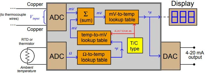
temperature transmitter.
Perhaps the greatest advantage of software compensation is the flexibility to easily switch between different thermocouple types with no hardware modification.
So long as the microprocessor memory is programmed with look-up tables relating voltage values to temperature values, it may accurately measure (and compensate for the reference junction of) any thermocouple type.
Hardware-based compensation schemes (e.g. an analog “ice point” circuit) require re-wiring or replacement to accommodate different thermocouple types, since each ice-point circuit is built to generate a compensating voltage for a specific type of thermocouple.
Side Effects of Reference Junction Compensation in Thermocouple
Reference junction compensation is a necessary part of any precision thermocouple circuit, due to the inescapable fact of the reference junction’s existence.
When you form a complete circuit of dissimilar metals, you will form both a measurement junction and a reference junction, with those two junctions’ polarities opposed to one another.
This is why reference junction compensation – whether it takes the form of a hardware circuit or an algorithm in software – must exist within every precision thermocouple instrument.
The presence of reference junction compensation in every precision thermocouple instrument results in an interesting phenomenon: if you directly short-circuit the thermocouple input terminals of such an instrument, it will always register ambient temperature, regardless of the thermocouple type the instrument is built or configured for.
This behavior may be illustrated by example, first showing a normal operating temperature measurement system and then with that same system short-circuited.
Here we see a temperature indicator receiving a 4-20 mA current signal from a temperature transmitter, which is receiving a millivoltage signal from a type “K” thermocouple sensing a process temperature of 780 degrees Fahrenheit:
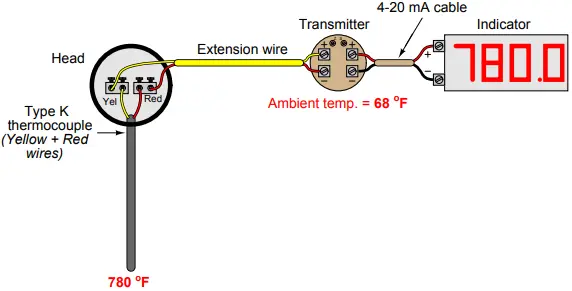
The transmitter’s internal reference junction compensation feature compensates for the ambient temperature of 68 degrees Fahrenheit.
If the ambient temperature rises or falls, the compensation will automatically adjust for the change in reference junction potential, such that the output will still register the process (measurement junction) temperature of 780 degrees F.
This is what the reference junction compensation is designed to do.
Now, we disconnect the thermocouple from the temperature transmitter and short-circuit the transmitter’s input:
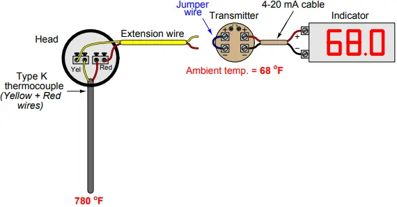
With the input short-circuited, the transmitter “sees” no voltage at all from the thermocouple circuit. There is no measurement junction nor a reference junction to compensate for, just a piece of wire making both input terminals electrically common.
This means the reference junction compensation inside the transmitter no longer performs a useful function. However, the transmitter does not “know” it is no longer connected to the thermocouple, so the compensation keeps on working even though it has nothing to compensate for.
Recall the voltage equation relating measurement, reference, and compensation voltages in a hardware-compensated thermocouple instrument: Vmeter = VJ1 − VJ2 + Vrjc
Disconnecting the thermocouple wire and connecting a shorting jumper to the instrument eliminates the VJ1 and VJ2 terms, leaving only the compensation voltage to be read by the meter:
Vmeter = 0 + Vrjc
Vmeter = Vrjc
This is why the instrument registers the equivalent temperature created by the reference junction compensation feature: this is the only signal it “sees” with its input short-circuited.
This phenomenon is true regardless of which thermocouple type the instrument is configured for, which makes it a convenient “quick test” of instrument function in the field.
If a technician short-circuits the input terminals of any thermocouple instrument, it should respond as though it is sensing ambient temperature.
While this interesting trait is a somewhat useful side-effect of reference junction compensation in thermocouple instruments, there are other effects that are not quite so useful.
The presence of reference junction compensation becomes quite troublesome, for example, if one tries to simulate a thermocouple using a precision millivoltage source.
Simply setting the millivoltage source to the value corresponding to the desired (simulation) temperature given in a thermocouple table will yield an incorrect result for any ambient temperature other than the freezing point of water!
Suppose, for example, a technician wished to simulate a type K thermocouple at 300 degrees Fahrenheit by setting a millivolt source to 6.094 millivolts (the voltage corresponding to 300 oF for type K thermocouples according to the ITS-90 standard).
Connecting the millivolt source to the instrument will not result in an instrument response appropriate for 300 degrees F:
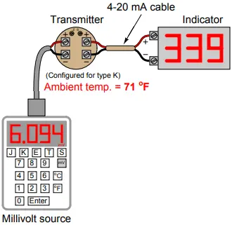
Instead, the instrument registers 339 degrees because its internal reference junction compensation feature is still active, compensating for a reference junction voltage that no longer exists.
The millivolt source’s output of 6.094 mV gets added to the compensation voltage (inside the transmitter) of 0.865 mV – the necessary millivolt value to compensate for a type K reference junction at 71 oF – with the result being a larger millivoltage (6.959 mV) interpreted by the transmitter as a temperature of 339 oF.
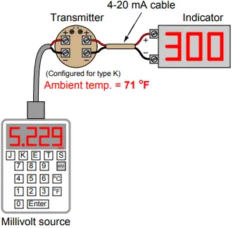
One way to use a millivoltage source to simulate a desired temperature is for the instrument technician to “out-think” the transmitter’s compensation feature by specifying a millivolt signal that is offset by the amount of equivalent voltage generated by the transmitter’s compensation.
In other words, instead of setting the millivolt source to a value of 6.094 mV, the technician should set the source to only 5.229 mV so the transmitter’s compensation will add 0.865 mV to this value to arrive at 6.094 mV and properly register as 300 degrees Fahrenheit:
Years ago, the only suitable piece of test equipment available for generating the precise millivoltage signals necessary to calibrate thermocouple instruments was a device called a precision potentiometer.
These “potentiometers” used a stable mercury cell battery (sometimes called a standard cell) as a voltage reference and a potentiometer with a calibrated knob to output low voltage signals.
Of course, modern thermocouple calibrators also provide direct entry of temperature and automatic compensation to “un-compensate” the transmitter such that any desired temperature may be easily simulated:
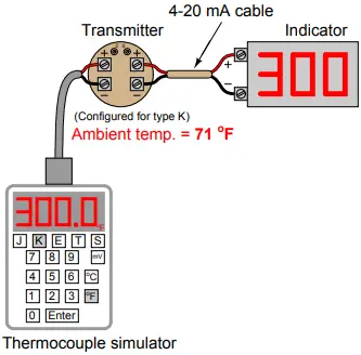
In this example, when the technician sets the calibrator for 300 oF (type K), it measures the ambient temperature and automatically subtracts 0.865 mV from the output signal, so only 5.229 mV is sent to the transmitter terminals instead of the full 6.094 mV.
The transmitter’s internal reference junction compensation adds the 0.865 mV offset value (thinking it must compensate for a reference junction that in reality is not there) and “sees” a total signal voltage of 6.094 mV, interpreting this properly as 300 degrees Fahrenheit.
The ITS-90 thermocouple standard declares a millivoltage signal value of 15.032 mV for a type S thermocouple junction at 2650 degrees F (with a reference junction temperature of 32 degrees F).
Note how the calibrator does not output 15.032 mV even though the simulated temperature has been set to 2650 degrees F. Instead, it outputs 14.910 mV, which is 0.122 mV less than 15.032 mV.
This offset of 0.122 mV corresponds to the calibrator’s local temperature of 70.8 degrees F (according to the ITS-90 standard for type S thermocouples).
When the calibrator’s 14.910 mV signal reaches the thermocouple instrument being calibrated (be it an indicator, transmitter, or even a controller equipped with a type S thermocouple input), the instrument’s own internal reference junction compensation will add 0.122 mV to the received signal of 14.910 mV, “thinking” it needs to compensate for a real reference junction.
The result will be a perceived measurement junction signal of 15.032 mV, which is exactly what we want the instrument to “think” it sees if our goal is to simulate connection to a real type S thermocouple at a temperature of 2650 degrees F.