Basic Principles of Venturi Tubes
The standard “textbook example” flow element used to create a pressure change by accelerating a fluid stream is the venturi tube: a pipe purposefully narrowed to create a region of low pressure.
As shown previously, venturi tubes are not the only structure capable of producing a flow-dependent pressure drop.
You should keep this in mind as we proceed to derive equations relating flow rate with pressure change: although the venturi tube is the canonical form, the exact same mathematical relationship applies to all flow elements generating a pressure drop by accelerating fluid, including orifice plates, flow nozzles, V-cones, segmental wedges, pipe elbows, pitot tubes, etc.
If the fluid going through the venturi tube is a liquid under relatively low pressure, we may vividly show the pressure at different points in the tube by means of piezometers, which are transparent tubes allowing us to view liquid column heights. The greater the height of liquid column in the piezometer, the greater the pressure at that point in the flowstream:
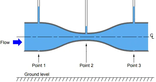
As indicated by the piezometer liquid heights, pressure at the constriction (point 2) is the least, while pressures at the wide portions of the venturi tube (points 1 and 3) are the greatest.
This is a counter-intuitive result, but it has a firm grounding in the physics of mass and energy conservation.
If we assume no energy is added (by a pump) or lost (due to friction) as fluid travels through this pipe, then the Law of Energy Conservation describes a situation where the fluid’s energy must remain constant at all points in the pipe as it travels through.
If we assume no fluid joins this flowstream from another pipe, or is lost from this pipe through any leaks, then the Law of Mass Conservation describes a situation where the fluid’s mass flow rate must remain constant at all points in the pipe as it travels through.
So long as fluid density remains fairly constant, fluid velocity must increase as the cross-sectional area of the pipe decreases, acording to the Law of Continuity:
This equation tells us that the ratio of fluid velocity between the narrow throat (point 2) and the wide mouth (point 1) of the pipe is the same ratio as the mouth’s area to the throat’s area.
So, if the mouth of the pipe had an area 5 times as great as the area of the throat, then we would expect the fluid velocity in the throat to be 5 times as great as the velocity at the mouth.
Simply put, the narrow throat causes the fluid to accelerate from a lower velocity to a higher velocity.
We know from our study of energy in physics that kinetic energy is proportional to the square of a mass’s velocity (Ek = mv2/2 ). If we know the fluid molecules increase velocity as they travel through the venturi tube’s throat, we may safely conclude that those molecules’ kinetic energies must increase as well.
However, we also know that the total energy at any point in the fluid stream must remain constant, because no energy is added to or taken away from the stream in this simple fluid system.
Therefore, if kinetic energy increases at the throat, potential energy must correspondingly decrease to keep the total amount of energy constant at any point in the fluid.
Potential energy may be manifest as height above ground, and/or as pressure in a fluid system. Since this venturi tube is level with the ground, there cannot be a height change to account for a change in potential energy.
Therefore, there must be a change of pressure (P) as the fluid travels through the venturi throat. The Laws of Mass and Energy Conservation invariably lead us to this conclusion: fluid pressure must decrease as it travels through the narrow throat of the venturi tube.
Conservation of energy at different points in a fluid stream is neatly expressed in Bernoulli’s Equation as a constant sum of elevation, pressure, and velocity “heads”:
z1ρg + v12ρ/2 + P1 = z2ρg + v22ρ/2 + P2
Where, z = height of fluid (from a common reference point, usually ground level), ρ = mass density of fluid, g = acceleration of gravity, v = velocity of fluid, P = Pressure of fluid.
We will use Bernoulli’s equation to develop a precise mathematical relationship between pressure and flow rate in a venturi tube. To simplify our task, we will hold to the following assumptions for our venturi tube system:
- No energy lost or gained in the venturi tube (all energy is conserved)
- No mass lost or gained in the venturi tube (all mass is conserved)
- Fluid is incompressible
- Venturi tube centerline is level (no height changes to consider)
Applying the last two assumptions to Bernoulli’s equation, we see that the “elevation head” term drops out of both sides, since z, ρ, and g are equal at all points in the system:
v12ρ/2 + P1 = v22ρ/2 + P2
Now we will algebraically re-arrange this equation to show pressures at points 1 and 2 in terms of velocities at points 1 and 2:
v22ρ/2 – v12ρ/2 = P1 – P2
(v22 – v12)ρ/2 = P1 – P2
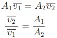
The Continuity equation shows us the relationship between velocities v1 and v2 and the areas at those points in the venturi tube, assuming constant density (ρ):
A1v1 = A2v2
Specifically, we need to re-arrange this equation to define v1 in terms of v2 so we may substitute into Bernoulli’s equation:
v1 = (A2/A1)/v2
Performing the algebraic substitution:
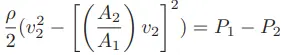
Solving for v2:
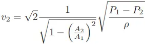
The result shows us how to solve for fluid velocity at the venturi throat (v2) based on a difference of pressure measured between the mouth and the throat (P1 − P2).
We are only one step away from a volumetric flow equation here, and that is to convert velocity (v) into flow rate (Q).
Velocity is expressed in units of length per time (feet or meters per second or minute), while volumetric flow is expressed in units of volume per time (cubic feet or cubic meters per second or minute).
We know that general flow/area/velocity relationship: Q = Av
Multiplying throat velocity (v2) by throat area (A2) and solving will give us the result we seek:
Volumetric Flow Calculations
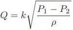
As we saw in the above section, we may derive a relatively simple equation for predicting flow through a fluid-accelerating element given the pressure drop generated by that element and the density of the fluid flowing through it.
Following equation is a simplified version of the equation 1:
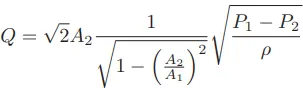
As you can see, the constant of proportionality (k) shown in the simpler equation is nothing more than a condensation of the first half of the longer equation: k represents the geometry of the venturi tube.
If we define k by the mouth and throat areas (A1, A2) of any particular venturi tube, we must be very careful to express the pressures and densities in compatible units of measurement.
For example, with k strictly defined by flow element geometry (tube areas measured in square feet), the calculated flow rate (Q) must be in units of cubic feet per second, the pressure values P1 and P2 must be in units of pounds per square foot, and mass density must be in units of slugs per cubic foot. We cannot arbitrarily choose different units of measurement for these variables, because the units must “agree” with one another.
If we wish to use more convenient units of measurement such as inches of water column for pressure and specific gravity (unitless) for density, the original (longer) equation simply will not work.
However, if we happen to know the differential pressure produced by any particular flow element tube with any particular fluid density at a specified flow rate (real-life conditions), we may calculate a value for k in the short equation that makes all those measurements “agree” with one another.
In other words, we may use the constant of proportionality (k) as a unit-of-measurement correction factor as well as a definition of element geometry.
This is a useful property of all proportionalities: simply insert values (expressed in any unit of measurement) determined by physical experiment and solve for the proportionality constant’s value to satisfy the expression as an equation.
If we do this, the value we arrive at for k will automatically compensate for whatever units of measurement we arbitrarily choose for pressure and density.
For example, if we know a particular orifice plate develops 45 inches of water column differential pressure at a flow rate of 180 gallons per minute of water (specific gravity = 1), we may insert these values into the equation 1 and solve for k:
180 = k √(45/1)
k = 26.83
Now we possess a value for k (26.83) that yields a flow rate in units of “gallons per minute” given differential pressure in units of “inches of water column” and density expressed as a specific gravity for this particular orifice plate.
From the known fact of all accelerating flow elements’ behavior (flow rate proportional to the square root of pressure divided by density) and from a set of values experimentally determined for this particular orifice plate, we now have an equation useful for calculating flow rate given any set of pressure and density values we may happen to encounter with this particular orifice plate:
gal/min = 26.83√(”W.C./Specific gravity)
This k value lets us predict flow for any given pressure difference – and vice-versa – for this particular orifice plate.
For example, if we wished to know the water flow rate corresponding to a pressure difference of 60 inches water column, we could use this equation to calculate a flow rate of 207.8 gallons per minute:
Q = 26.83√(60/1)
Q = 207.8 GPM
As another example, a measured differential pressure of 110 inches water column across this orifice plate generated by a flow of gasoline (specific gravity = 0.657) would correspond to a gasoline flow rate of 347 gallons per minute:
Q = 26.83√(110/0.657)
Q = 347 GPM
Suppose, though, we wished to have an equation for calculating the flow rate through this same orifice plate given pressure and density data in different units (say, kPa instead of inches water column, and kilograms per cubic meter instead of specific gravity).
In order to do this, we would need to re-calculate the constant of proportionality (k) to accommodate those new units of measurement.
To do this, all we would need is a single set of experimental data for the orifice plate relating flow in GPM, pressure in kPa, and density in kg/m3 .
Applying this to our original data where a water flow rate of 180 GPM resulted in a pressure drop of 45 inches water column, we could convert the pressure drop of 45 ”W.C. into 11.21 kPa and express the density as 1000 kg/m3 to solve for a new value of k:
180 = k√(11.21/1000)
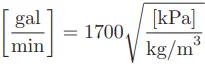
k = 1700
Nothing about the orifice plate’s geometry has changed from before, only the units of measurement we have chosen to work with.
Now we possess a value for k (1700) for the same orifice plate yielding a flow rate in units of “gallons per minute” given differential pressure in units of “kilopascals” and density in units of “kilograms per cubic meter.”
If we were to be given a pressure drop in kPa and a fluid density in kg/m3 for this orifice plate, we could calculate the corresponding flow rate (in GPM) with our new value of k (1700) just as easily as we could with the old value of k (26.83) given pressure in ”W.C. and specific gravity.
Mass Flow Calculations
Measurements of mass flow are preferred over measurements of volumetric flow in process applications where mass balance (monitoring the rates of mass entry and exit for a process) is important.
Whereas volumetric flow measurements express the fluid flow rate in such terms as gallons per minute or cubic meters per second, mass flow measurements always express fluid flow rate in terms of actual mass units over time, such pounds (mass) per second or kilograms per minute.
Applications for mass flow measurement include custody transfer (where a fluid product is bought or sold by its mass), chemical reaction processes (where the mass flow rates of reactants must be maintained in precise proportion in order for the desired chemical reactions to occur), and steam boiler control systems.
(where the out-flow of vaporous steam must be balanced by an equivalent in-flow of liquid water to the boiler – here, volumetric comparisons of steam and water flow would be useless because one cubic foot of steam is certainly not the same number of H2O molecules as one cubic foot of water)
If we wish to calculate mass flow instead of volumetric flow, the equation does not change much. The relationship between volume (V ) and mass (m) for a sample of fluid is its mass density (ρ):
ρ = m/V
Similarly, the relationship between a volumetric flow rate (Q) and a mass flow rate (W) is also the fluid’s mass density (ρ):
ρ = W/Q
Solving for W in this equation leads us to a product of volumetric flow rate and mass density: W = ρQ
To turn our general volumetric flow equation into a mass flow equation multiply both sides by fluid density (ρ):
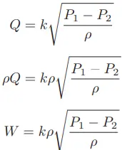
After simplfying the above mass flow equation we will get:
As with the volumetric flow equation, all we need in order to arrive at a suitable k value for any particular flow element is a set of values taken from that real element in service, expressed in whatever units of measurement we desire.
For example, if we had a venturi tube generating a differential pressure of 2.30 kilopascals (kPa) at a mass flow rate of 500 kilograms per minute of naphtha (a petroleum product having a density of 0.665 kilograms per liter), we could solve for the k value of this venturi tube as such:
500 = k√ (0.665 x 2.3)
k = 404.3
Now that we know a value of 404.3 for k will yield kilograms per minute of liquid flow through this venturi tube given pressure in kPa and density in kilograms per liter, we may readily predict the mass flow rate through this tube for any other pressure drop and fluid density we might happen to encounter. The value of 404.3 for k relates the disparate units of measurement for us:
kg/min = 404.3√[(kg/1)(kgPa)]
As with volumetric flow calculations, the calculated value for k neatly accounts for any set of measurement units we may arbitrarily choose. The key is first knowing the proportional relationship between flow rate, pressure drop, and density.
Once we combine that proportionality with a specific set of data experimentally gathered from a particular flow element, we have a true equation properly relating all the variables together in our chosen units of measurement.
If we happened to measure 6.1 kPa of differential pressure across this same venturi tube as it flowed sea water (density = 1.03 kilograms per liter), we could calculate the mass flow rate quite easily using the same equation (with the k factor of 404.3):
W = 404.3 √(1.03 x 6.1)
W = 1013.4 kg/min